Milton Crash Data Analysis
[1]:
import pandas as pd
import folium
import geopandas as gpd
from shapely.geometry import Point
import matplotlib.pyplot as plt
import contextily as ctx
import milton_maps as mm
import seaborn as sns
import logging

from milton_maps.process_crash_data import *

logging.basicConfig(level=logging.INFO)
logger = logging.getLogger("notebook")

# Suppress warnings in notebook output
import warnings
warnings.filterwarnings('ignore')
/Users/alexhasha/Library/Caches/pypoetry/virtualenvs/milton-maps-gfMaDXEA-py3.11/lib/python3.11/site-packages/geopandas/_compat.py:123: UserWarning: The Shapely GEOS version (3.10.3-CAPI-1.16.1) is incompatible with the GEOS version PyGEOS was compiled with (3.10.4-CAPI-1.16.2). Conversions between both will be slow.
  warnings.warn(
[2]:
milton_boundaries = get_milton_boundaries()
[3]:
crash_geodf = get_crash_data()
INFO:process_crash_data:Found 2173 records missing coordinates, and will be dropped
INFO:process_crash_data:Found 555 records outside Milton were dropped by the geoclip.
[4]:
crash_geodf.columns
[4]:
Index(['Crash_Number', 'City_Town_Name', 'Crash_Date', 'Crash_Time',
       'Crash_Severity', 'Maximum_Injury_Severity_Reported',
       'Number_of_Vehicles', 'Total_Nonfatal_Injuries', 'Total_Fatal_Injuries',
       'Manner_of_Collision', 'Vehicle_Action_Prior_to_Crash',
       'Vehicle_Travel_Directions', 'Most_Harmful_Events',
       'Vehicle_Configuration', 'Road_Surface_Condition', 'Ambient_Light',
       'Weather_Condition', 'At_Roadway_Intersection',
       'Distance_From_Nearest_Roadway_Intersection',
       'Distance_From_Nearest_Milemarker', 'Distance_From_Nearest_Exit',
       'Distance_From_Nearest_Landmark', 'Non_Motorist_Type', 'X_Cooordinate',
       'Y_Cooordinate', 'Crash_DateTime', 'year', 'severity', 'geometry'],
      dtype='object')
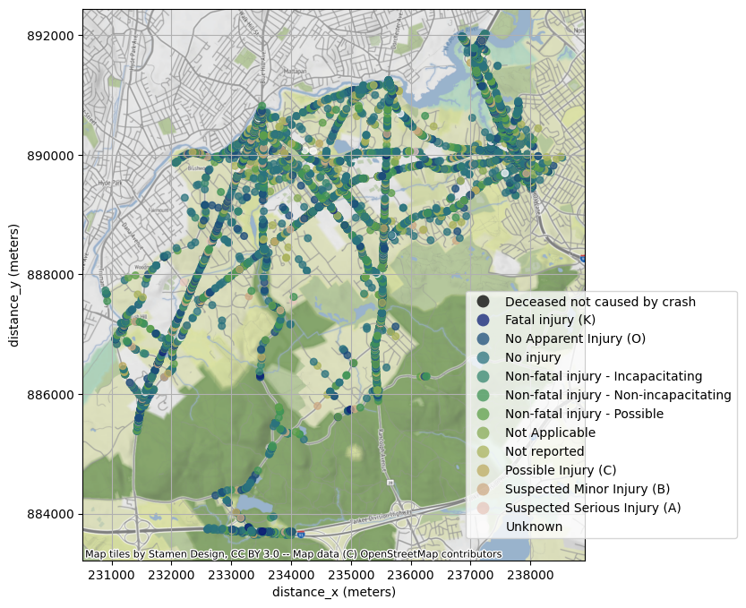
Visualize crash locations to help verify filtering logic
[5]:
fig, ax = plt.subplots(1, figsize=(8,8))
# Tighten the bounding box around the data locations
ax = mm.plot_map(crash_geodf,
                 column="Maximum_Injury_Severity_Reported",
                 categorical=True,
                 markersize=30,
                 alpha=0.75,
                 ax=ax,
                 )
# Move legend to the bottom right
ax.get_legend().set_bbox_to_anchor((.75, 0.5))
ctx.add_basemap(ax, crs="EPSG:26986")
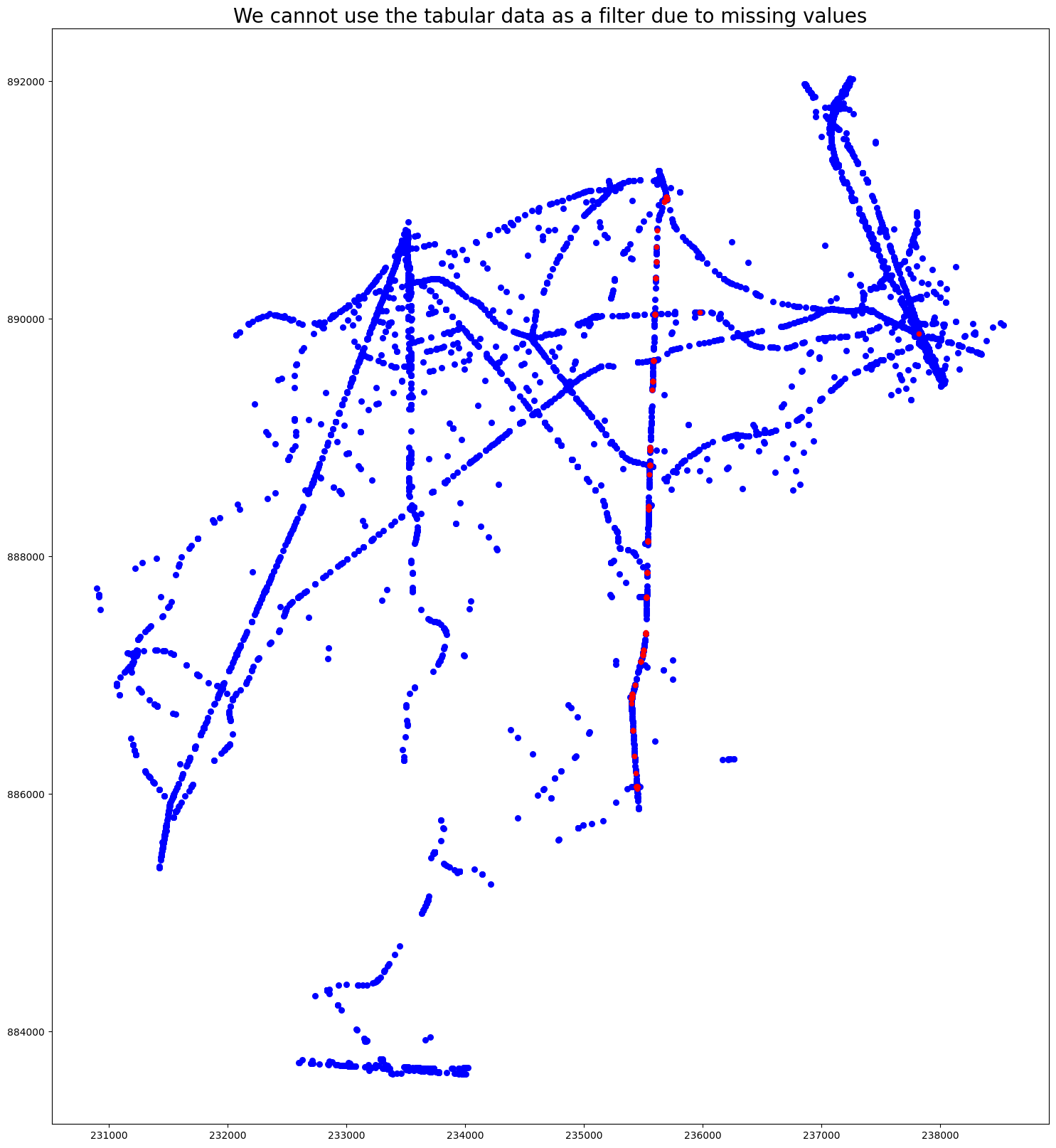
Question: How to identify accidents along Randolph Avenue?
Unsuccessfull approach: filtering on tabular metadata
[6]:
crash_geodf["At_Roadway_Intersection"].value_counts()
[6]:
At_Roadway_Intersection
RANDOLPH AVENUE / CHICKATAWBUT ROAD                                                 81
GRANITE AVENUE / SQUANTUM STREET                                                    59
BROOK ROAD / CENTRE STREET                                                          40
GRANITE AVENUE / ADAMS STREET                                                       31
RANDOLPH AVENUE / BROOK ROAD                                                        28
                                                                                    ..
BLUE HILL AVENUE / BLUE HILL AVENUE / BRUSH HILL ROAD                                0
RANDOLPH AVENUE / REEDSDALE ROAD Rte  / Randolph Ave Rte 28 N / Reedsdale Rd Rte     0
Rte 138 N / BLUE HILL AVENUE                                                         0
RANDOLPH AVENUE / REEDSDALE ROAD Rte  / Randolph Ave Rte N / Reedsdale Rd Rte        0
/                                                                                    0
Name: count, Length: 2204, dtype: int64
[7]:
crash_geodf.loc[
    crash_geodf["At_Roadway_Intersection"].str.lower().str.contains("randolph").fillna(False),
    "At_Roadway_Intersection"
].value_counts()
[7]:
At_Roadway_Intersection
RANDOLPH AVENUE / CHICKATAWBUT ROAD                  81
RANDOLPH AVENUE / BROOK ROAD                         28
RANDOLPH AVENUE Rte 28 N / CHICKATAWBUT ROAD         26
RANDOLPH AVENUE / REEDSDALE ROAD                     23
RANDOLPH AVENUE Rte 28 / CHICKATAWBUT ROAD           22
                                                     ..
BROOK ROAD / FAIRFAX ROAD                             0
BROOK ROAD / DUDLEY LANE                              0
BROOK ROAD / CHURCHILL LANE                           0
BROOK ROAD / CENTRE STREET / CENTRE ST / BROOK RD     0
\ / GRANITE AVENUE / GRANITE AVENUE                   0
Name: count, Length: 2204, dtype: int64
[8]:
crash_geodf.shape
[8]:
(11602, 29)
[9]:
# Filter to crashes that occured on randolph using the pattern above.
randolph_crashes = crash_geodf.loc[crash_geodf["At_Roadway_Intersection"].str.lower().str.contains("randolph").fillna(False), :]
randolph_crashes.shape
[9]:
(805, 29)
[10]:
non_randolph_crashes = crash_geodf.loc[~crash_geodf["At_Roadway_Intersection"].str.lower().str.contains("randolph").fillna(False), :]
non_randolph_crashes.shape
[10]:
(10797, 29)
[11]:
# Plot randolph crashses in red and non-randolph crashes in blue
fig, ax = plt.subplots(1, figsize=(20,20))

non_randolph_crashes.plot(
    ax=ax,
    color="blue",
    markersize=30,
)

randolph_crashes.plot(
    ax=ax,
    color="red",
    markersize=20,
)

#Set plot title to "We cannot use the tabular data as a filter due to missing values"
#increase the size of the title to 20
ax.set_title("We cannot use the tabular data as a filter due to missing values", fontsize=20)
plt.show()
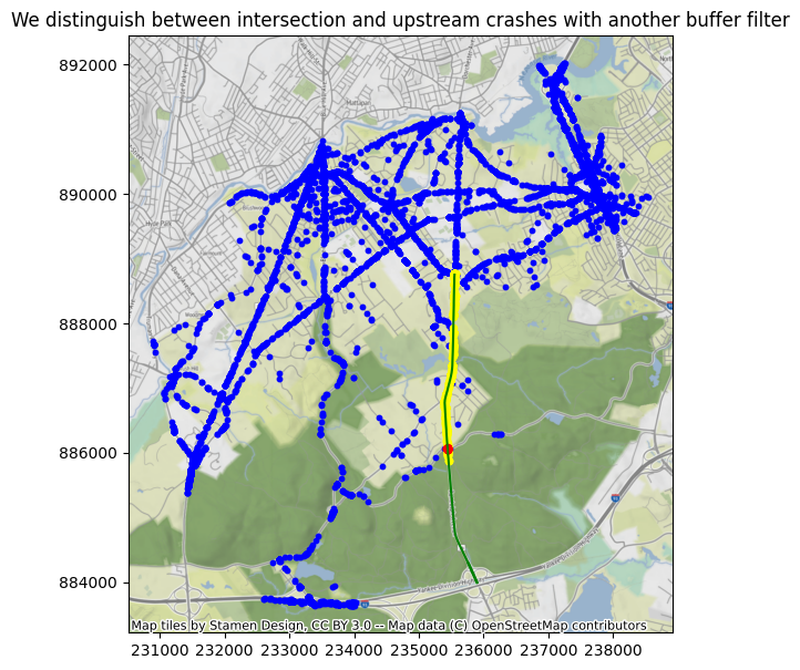
Successful approach: create bounding box from MassDOT road geometries.
[12]:
randolph_ave = get_randolph_ave_shape()
[13]:
intersection_crashes, upstream_crashes, randolph_ave_crashes = randolph_ave_upstream_vs_intersection(crash_geodf, randolph_ave)
other_crashes = crash_geodf.loc[~crash_geodf.index.isin(set(randolph_ave_crashes.index))]
INFO:process_crash_data:Intersection crashes shape: (413, 29)
INFO:process_crash_data:Upstream crashes shape: (767, 29)
[14]:
# Plot randolph crashses in red and non-randolph crashes in blue
fig, ax = plt.subplots(1, figsize=(7,7))

other_crashes.plot(
    ax=ax,
    color="blue",
    markersize=10,
)

upstream_crashes.plot(
    ax=ax,
    color="yellow",
    markersize=20,
)

intersection_crashes.plot(
    ax=ax,
    color="red",
    markersize=20,
)

randolph_ave.plot(
    ax=ax,
    color="green",
)

#Set plot title to "We cannot use the tabular data as a filter due to missing values"
#increase the size of the title to 20
ax.set_title("We distinguish between intersection and upstream crashes with another buffer filter", fontsize=12)
ctx.add_basemap(ax=ax, crs="EPSG:26986")
plt.show()
Make an interactive map of Randolph Ave crashes with popups giving more details on the crash
[30]:
def popup_text(row):
    result = f"""
    Direction of Travel: {row['Vehicle_Travel_Directions']}<br>
    Year: {row['year']}<br>
    Time of Day: {row['Crash_Time']}<br>
    Severity: {row['severity']}<br>
    Where: {row['where']}<br>
    """
    return result
[31]:
randolph_ave_crashes["severity"].value_counts(ascending=True)
[31]:
severity
Fatal Injury      7
Major Injury     36
Unknown          77
Minor Injury    454
No Injury       606
Name: count, dtype: int64
[32]:
# Create an interactive Folium Map with the crash points plotted and a popup with the direction of travel, time of day, and severity of the crash.  Color the points by severity of the crash
m = folium.Map(location=[42.224225, -71.070639], zoom_start=18)
# Create a version of randolph_ave_crashes that uses a CRS in latitude and longitude
randolph_ave_crashes_latlon = randolph_ave_crashes.to_crs("EPSG:4326")

injury_crashes = randolph_ave_crashes_latlon.loc[
    randolph_ave_crashes_latlon["severity"].isin(
        ["Fatal Injury", "Major Injury", "Minor Injury"]), :]

colormap = {
    "Fatal Injury": "red",
    "Major Injury": "yellow",
    "Minor Injury": "blue",
}


for _, row in injury_crashes.sort_values(by="severity", ascending=False).iterrows():
    popup_content = folium.Popup(popup_text(row), max_width=300)  # Adjust max_width as needed
    folium.CircleMarker(
        location=[row["geometry"].y, row["geometry"].x],
        radius=5,
        popup=popup_content,
        color=colormap[row["severity"]],
        fill=True,
        fill_color="yellow",
        fill_opacity=0.5,
    ).add_to(m)

display(m)
Make this Notebook Trusted to load map: File -> Trust Notebook
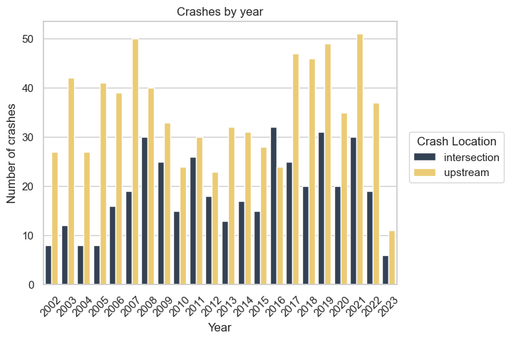
Create a structured dataframe of intersection vs upstream crashes
[ ]:
[18]:
intersection_crashes["where"] = "intersection"
upstream_crashes["where"] = "upstream"
randolph_ave_crashes = gpd.GeoDataFrame( pd.concat([intersection_crashes, upstream_crashes], ignore_index=True) )
[19]:
# Use seaborn to plot number of crashes by year colored by "where"
sns.set_theme(style="whitegrid")
sns.set_palette(["#2d4059", "#ffd460"])
ax = sns.countplot(x="year", hue="where", data=randolph_ave_crashes)
ax.set_title("Crashes by year")
ax.set_ylabel("Number of crashes")
ax.set_xlabel("Year")
# Rotate x axis labels 45 degrees
plt.xticks(rotation=45)
leg = ax.legend()
leg.set_title("Crash Location")
leg.set_bbox_to_anchor((1.02, .6))

plt.show()
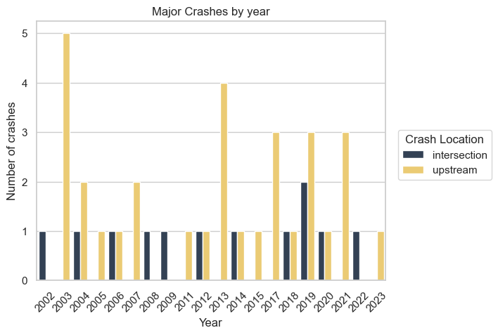
[20]:
# Apply the following color palette to the plot below:
# intersection: #2d4059
# upstream: #ffd460
sns.set_theme(style="whitegrid")
sns.set_palette(["#2d4059", "#ffd460"])
_data = randolph_ave_crashes.loc[randolph_ave_crashes["severity"].isin(["Major Injury", "Fatal Injury"])]
ax = sns.countplot(x="year", hue="where", data=_data)
ax.set_title("Major Crashes by year")
ax.set_ylabel("Number of crashes")
ax.set_xlabel("Year")
# Rotate x axis labels 45 degrees
plt.xticks(rotation=45)
leg = ax.legend()
leg.set_title("Crash Location")
leg.set_bbox_to_anchor((1.02, .6))

plt.show()
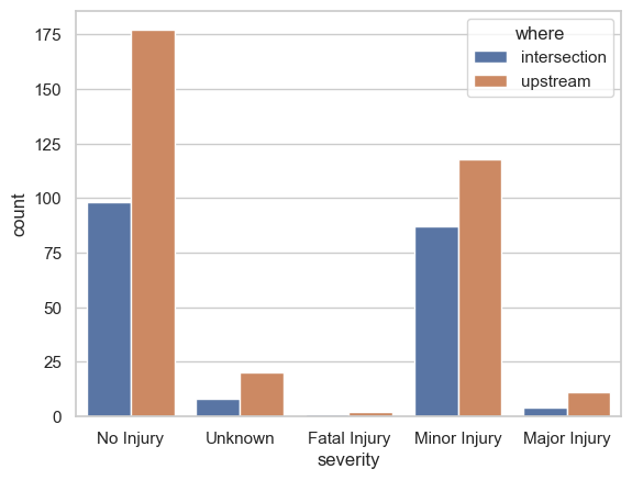
[21]:
# Use seaborn to plot number of crashes by severity, colored by "where", over the last 4 years
sns.set_theme(style="whitegrid")
ax = sns.countplot(x="severity", hue="where", data=randolph_ave_crashes[randolph_ave_crashes.year >= 2015])
[22]:
randolph_ave_crashes[randolph_ave_crashes.year >= 2010].groupby(["severity", "where"]).size()
[22]:
severity      where
Fatal Injury  intersection      2
              upstream          4
Major Injury  intersection      5
              upstream         16
Minor Injury  intersection    130
              upstream        171
No Injury     intersection    135
              upstream        250
Unknown       intersection     15
              upstream         27
dtype: int64
[23]:
randolph_ave_crashes.columns
[23]:
Index(['Crash_Number', 'City_Town_Name', 'Crash_Date', 'Crash_Time',
       'Crash_Severity', 'Maximum_Injury_Severity_Reported',
       'Number_of_Vehicles', 'Total_Nonfatal_Injuries', 'Total_Fatal_Injuries',
       'Manner_of_Collision', 'Vehicle_Action_Prior_to_Crash',
       'Vehicle_Travel_Directions', 'Most_Harmful_Events',
       'Vehicle_Configuration', 'Road_Surface_Condition', 'Ambient_Light',
       'Weather_Condition', 'At_Roadway_Intersection',
       'Distance_From_Nearest_Roadway_Intersection',
       'Distance_From_Nearest_Milemarker', 'Distance_From_Nearest_Exit',
       'Distance_From_Nearest_Landmark', 'Non_Motorist_Type', 'X_Cooordinate',
       'Y_Cooordinate', 'Crash_DateTime', 'year', 'severity', 'geometry',
       'where'],
      dtype='object')
[24]:
randolph_ave_crashes.loc[
    randolph_ave_crashes.severity == "Fatal Injury",
    ["Crash_DateTime", "where", "Crash_Date", "Crash_Time", "Manner_of_Collision", "Number_of_Vehicles", "Total_Fatal_Injuries", "Ambient_Light", "Weather_Condition"]
].sort_values(by="Crash_DateTime", ascending=False).drop(columns=["Crash_DateTime"])
[24]:
| where | Crash_Date | Crash_Time | Manner_of_Collision | Number_of_Vehicles | Total_Fatal_Injuries | Ambient_Light | Weather_Condition | |
|---|---|---|---|---|---|---|---|---|
| 3 | intersection | 15-Jul-2022 | 10:30 PM | Not reported | 2 | 1 | Not reported | Not Reported |
| 870 | upstream | 31-Aug-2017 | 8:42 AM | Angle | 2 | 1 | Daylight | Clear |
| 772 | upstream | 25-Apr-2017 | 4:03 PM | Head-on | 2 | 1 | Daylight | Rain/Cloudy |
| 204 | intersection | 31-May-2014 | 1:49 AM | Single vehicle crash | 1 | 1 | Dark - lighted roadway | Clear/Clear |
| 678 | upstream | 28-Nov-2013 | 7:55 AM | Single vehicle crash | 1 | 1 | Daylight | Clear |
| 731 | upstream | 01-Nov-2012 | 6:22 PM | Single vehicle crash | 1 | 1 | Dark - lighted roadway | Clear/Unknown |
| 919 | upstream | 15-Feb-2005 | 12:05 PM | Sideswipe, opposite direction | 2 | 1 | Daylight | Clear |
[25]:
# From 2014 to 2016 there were 54 crashes at this intersection. Of those 54, 28 involved a fatality or injury.
intersection_crashes.loc[
    (intersection_crashes.year >= 2014) &
    (intersection_crashes.year <= 2016)].shape[0]
[25]:
(64, 30)
[26]:
intersection_crashes.loc[
    (intersection_crashes.year >= 2014) &
    (intersection_crashes.year <= 2016), "severity"].value_counts()
[26]:
severity
Minor Injury    30
No Injury       30
Unknown          3
Fatal Injury     1
Name: count, dtype: int64
Scratch
[ ]:
[ ]:
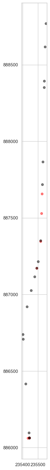
[27]:
# Expand the axes of this plot to match the range of data in crash_geodf2
fig, ax = plt.subplots(1, figsize=(20,20))
randolph_ave_crashes.loc[
    (randolph_ave_crashes.year >= 2010) & (randolph_ave_crashes.severity.isin(["Fatal Injury", "Major Injury"])),
].plot(
    ax=ax,
    column="severity",
    categorical=True,
    markersize=30,
    alpha=0.5,
    cmap = "flag"
)
# x and y range in crash_geodf
xmin = crash_geodf2.geometry.x.min()
xmax = crash_geodf2.geometry.x.max()
ymin = crash_geodf2.geometry.y.min()
ymax = crash_geodf2.geometry.y.max()
ax.set_xlim(xmin, xmax)
ax.set_ylim(ymin, ymax)

ctx.add_basemap(ax, crs="EPSG:26986")
plt.show()
---------------------------------------------------------------------------
NameError                                 Traceback (most recent call last)
/Users/alexhasha/repos/milton_maps/notebooks/crash_analysis.ipynb Cell 38 line 1
      <a href='vscode-notebook-cell:/Users/alexhasha/repos/milton_maps/notebooks/crash_analysis.ipynb#Z1450sZmlsZQ%3D%3D?line=2'>3</a> randolph_ave_crashes.loc[
      <a href='vscode-notebook-cell:/Users/alexhasha/repos/milton_maps/notebooks/crash_analysis.ipynb#Z1450sZmlsZQ%3D%3D?line=3'>4</a>     (randolph_ave_crashes.year >= 2010) & (randolph_ave_crashes.severity.isin(["Fatal Injury", "Major Injury"])),
      <a href='vscode-notebook-cell:/Users/alexhasha/repos/milton_maps/notebooks/crash_analysis.ipynb#Z1450sZmlsZQ%3D%3D?line=4'>5</a> ].plot(
   (...)
     <a href='vscode-notebook-cell:/Users/alexhasha/repos/milton_maps/notebooks/crash_analysis.ipynb#Z1450sZmlsZQ%3D%3D?line=10'>11</a>     cmap = "flag"
     <a href='vscode-notebook-cell:/Users/alexhasha/repos/milton_maps/notebooks/crash_analysis.ipynb#Z1450sZmlsZQ%3D%3D?line=11'>12</a> )
     <a href='vscode-notebook-cell:/Users/alexhasha/repos/milton_maps/notebooks/crash_analysis.ipynb#Z1450sZmlsZQ%3D%3D?line=12'>13</a> # x and y range in crash_geodf
---> <a href='vscode-notebook-cell:/Users/alexhasha/repos/milton_maps/notebooks/crash_analysis.ipynb#Z1450sZmlsZQ%3D%3D?line=13'>14</a> xmin = crash_geodf2.geometry.x.min()
     <a href='vscode-notebook-cell:/Users/alexhasha/repos/milton_maps/notebooks/crash_analysis.ipynb#Z1450sZmlsZQ%3D%3D?line=14'>15</a> xmax = crash_geodf2.geometry.x.max()
     <a href='vscode-notebook-cell:/Users/alexhasha/repos/milton_maps/notebooks/crash_analysis.ipynb#Z1450sZmlsZQ%3D%3D?line=15'>16</a> ymin = crash_geodf2.geometry.y.min()

NameError: name 'crash_geodf2' is not defined
[ ]:
import numpy as np

# Create a new dataframe for crashes from 2010 and with relevant 'severity' levels
filtered_crashes = randolph_ave_crashes.loc[
    (randolph_ave_crashes.year >= 2010)
]

# Convert geometry points to a NumPy array (needed for scikit-learn)
coords = filtered_crashes.geometry.apply(lambda p: [p.x, p.y]).to_list()
coords = np.array(coords)
[ ]:
min(coords[:,0])
[ ]:
from scipy.spatial import KDTree
import numpy as np
import matplotlib.pyplot as plt

# Example coords array; replace with your actual data
# coords = np.array([[x1, y1], [x2, y2], ...])

# Create a KDTree for efficient nearest neighbor search
kdtree = KDTree(coords)

# Define your curve parameterization here
# For example, let's assume a simple linear parameterization along the x-axis:
curve_y = np.linspace(min(coords[:,1]), max(coords[:,1]), 100)  # 100 equidistant points

# Initialize an array to hold counts of nearest points to each interval center
counts = np.zeros(curve.shape)

# Calculate the nearest crash point for each point along the curve
for i, x in enumerate(curve):
    # Query the KDTree for the nearest point
    distance, index = kdtree.query([x, 0])  # replace 0 with the corresponding y value on the curve
    # Increment the count for the nearest point
    counts[i] += 1

# Now 'counts' contains the number of times each point along the curve was the nearest point to a crash

# To visualize, let's plot the curve and color it based on 'counts'
plt.scatter(curve, np.zeros(curve.shape), c=counts, cmap='hot')
plt.colorbar(label='Number of nearest crashes')
plt.show()
[ ]:
from shapely.ops import linemerge

# Combine the LineStrings into a single MultiLineString
multi_line = linemerge(randolph_ave.geometry.tolist())
[ ]:
# Number of points you want along the curve
num_points = 100

# Calculate the length of the merged line
line_length = multi_line.length

# Calculate equally spaced distances along the line
distances = np.linspace(0, line_length, num_points)

# Create a list to hold the equally spaced points
equally_spaced_points = []

for distance in distances:
    # Use the `interpolate` method to find the point at each distance
    point = multi_line.interpolate(distance)
    equally_spaced_points.append(point)
[ ]:
equally_spaced_points
[ ]:
from scipy.spatial import KDTree
import numpy as np

# Create a KDTree from the equally spaced points
equally_spaced_coords = [(point.x, point.y) for point in equally_spaced_points]
kdtree = KDTree(equally_spaced_coords)

# Initialize an array to hold counts of nearest road points for each crash
counts = np.zeros(len(equally_spaced_points))

# Query KDTree for each crash point
crash_coords = filtered_crashes.geometry.apply(lambda p: (p.x, p.y)).tolist()
for coord in crash_coords:
    distance, index = kdtree.query(coord)
    counts[index] += 1

# Now 'counts' contains the number of times each equally spaced point along the road
# is the nearest point to a crash.

# You can visualize this data as needed.
[ ]:
counts
[ ]:
np.log10(counts+1)
[ ]:
# Scatter plot coords on a map, with markersize scaled by counts
fig, ax = plt.subplots(1, figsize=(20,20))
ax.scatter(
    x=[p.x for p in equally_spaced_points],
    y=[p.y for p in equally_spaced_points],
    s=np.log(counts+1)*30,
    alpha=0.5,
    color="red",
)
# Set equal aspect ratio
ax.set_aspect('equal', 'box')
[ ]:
index
[ ]:
crash_geodf['crash_time'] = pd.to_datetime(crash_geodf['Crash Date'] + " " + crash_geodf['Crash Time'])
[ ]:
crash_geodf.info()
[ ]:
roads_df = gpd.read_file("../data/raw/MassDOT_Roads_SHP/EOTMAJROADS_RTE_MAJOR.shp")
[ ]:
ax = roads_df[roads_df.RT_NUMBER=="28"].plot()
ctx.add_basemap(ax, crs="EPSG:26986")
[ ]:
rt28 = roads_df[roads_df.RT_NUMBER=="28"]
milton_rt_28 = gpd.clip(rt28, milton_boundaries)
ax = milton_rt_28.plot()
ctx.add_basemap(ax, crs="EPSG:26986")
[ ]:
[ ]:
df_nearest_major_road = gpd.sjoin_nearest(crash_geodf, roads_df, how="left", distance_col="distance_to_major_road")
[ ]:
df_nearest_major_road.info()
[ ]:
rt_28_crashes = df_nearest_major_road[(df_nearest_major_road.RT_NUMBER=="28") & (df_nearest_major_road.distance_to_major_road < 10.0)]
rt_28_crashes
[ ]:
ax = rt_28_crashes.plot(column="severity")
ctx.add_basemap(ax, crs="EPSG:26986")
[ ]:
rt_28_crashes['month_year'] = rt_28_crashes['crash_time'].dt.to_period('M')
[ ]:
df = rt_28_crashes.groupby(["month_year", "severity"])['RMV Crash Number'].count().reset_index()
df
[ ]:
#df.columns
accidents_over_time = df.pivot(index='month_year', columns='severity', values='RMV Crash Number').fillna(0)
[ ]:
accidents_over_time.plot.area()
[ ]:
milton_roads_df = gpd.read_file("../data/raw/MassDOT_Roads_SHP/EOTROADS_ARC.shp", mask=milton_boundaries)
ax = milton_roads_df.plot()
ctx.add_basemap(ax,crs="EPSG:26986")
[ ]:
milton_roads_df.head()
[ ]:
chickatawbut_road = milton_roads_df[milton_roads_df.STREETNAME=="CHICKATAWBUT ROAD"].dissolve()
chickatawbut_road.plot()
[ ]:
chickatawbut_road.dissolve().plot()
[ ]:
randolph_ave = milton_roads_df[milton_roads_df.STREETNAME=="RANDOLPH AVENUE"].dissolve()
randolph_ave.plot()
[ ]:
pd.concat([randolph_ave, chickatawbut_road]).plot()
[ ]:
randolph_chickatawbut_intsct = randolph_ave.geometry.intersection(chickatawbut_road.geometry).buffer(50)
ax = pd.concat([randolph_ave, chickatawbut_road]).plot()
ax = randolph_chickatawbut_intsct.plot(ax=ax)
ctx.add_basemap(ax, crs="EPSG:26986")
[ ]:
ax = randolph_chickatawbut_intsct.plot()
ctx.add_basemap(ax, crs="EPSG:26986", zoom=12)
[ ]:
randolph_chickatawbut_intsct
[ ]:
193.18/647
[ ]: